Written Exam |
The exam consists of answers to a number of tasks divided into subtasks, which are to be handed in electronically in http://e-learn.sdu.dk (Blackboard).
A small firm that produces two types of mattresses, Single and Double, has two workers for the final treatment of the mattresses before being ready for sell. In one hour the two workers can process the following number of mattresses:
The market demands at least 30 Single and 20 Double mattresses per day. The cost of one hour of working time is 90 Dkk for worker A and 80 Dkk for worker B. The management of the firm wants to determine the number of hours per day that each worker has to be engaged in order to meet the demand at the minimum cost. Workers can only be engaged for multiples of hours and not for fractions of hours.
Formulate the problem as an integer linear programming problem. (Ignore that workers can have a maximum number of working hours per day.)
Solution
|
In GLPK:
var x_1 integer >=  0;
var x_2 integer >=  0;
var x_3 integer >=  0;

minimize z:  90 * x_A  +  80 * x_B ;

subject to
 S:          3 *x_A  +  2 *x_B       >=  30;
 D:              x_A  +    2* x_B    >=  20;
solve;
end;
Write the linear programming relaxation (P1) of the original problem formulation (P) given at the previous subtask.
Explain the relation between the optimal solution of (P1) and the optimal solution of (P).
Solution
|
zLP is a lower bound of z.
Derive the dual (D1) of (P1) using the Lagrange multipliers approach. Show all steps of the derivation and write the final problem (D1).
Solution
We introduce the multipliers y1,y2≤ 0 and relax the two
constraints in the objective function:
| P(y1,y2)= min90 xA + 80 xB + y1 (3 xA +2 xB − 30) + y2 ( xA + 2 xB −20) |
Thus
| ∀ y1,y2≤ 0 P(y1,y2)≤ z |
Hence P(y1,y2) is a lower bound for P1. The best lower bound will be given by
|
The optimization problem
| c1x1+c2x2+…+cnxn |
can be solved by inspection as follows:
|
Hence the best lower bound will be:
|
or equivalently
|
Solution
After introduction of surplus variables by means of which we transform
the two constraints in equalities preserving positive right hand side
terms we obtain the first tableau.
Tableau #1
|-----+-----+----+----+----+----|
| x_A | x_B | s1 | s2 | -z |  b |
|-----+-----+----+----+----+----|
|   3 |   2 | -1 |  0 |  0 | 30 |
|   1 |   2 |  0 | -1 |  0 | 20 |
|  90 |  80 |  0 |  0 |  1 |  0 |
|-----+-----+----+----+----+----|
The canonical form has the identity matrix as a submatrix of the constraint matrix. We obtain it from the first tableau by multiplying by -1 the first and second row.
Tableau #2
|-----+-----+----+----+----+-----|
| x_A | x_B | s1 | s2 | -z |   b |
|-----+-----+----+----+----+-----|
|  -3 |  -2 |  1 |  0 |  0 | -30 |
|  -1 |  -2 |  0 |  1 |  0 | -20 |
|  90 |  80 |  0 |  0 |  1 |   0 |
|-----+-----+----+----+----+-----|
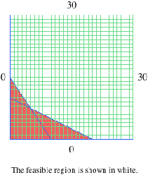
Since the RHS terms are negative the basic solution corresponding to this tableau is infeasible (surplus and slack variables are always defined to be non-negative).
Figure 1 shows the feasibility region graphically.
After two iterations of the appropriate form of the simplex method we obtain the two following tableaux:
Tableau #4
|-----+-----+------+------+----+----+------|
|     | x_A | x_B  | s1   | s2 | -z |    b |
|-----+-----+------+------+----+----+------|
| I   |   1 | 2/3  | -1/3 |  0 |  0 |   10 |
| II  |   0 | -4/3 | -1/3 |  1 |  0 |  -10 |
| III |   0 | 20   | 30   |  0 |  1 | -900 |
|-----+-----+------+------+----+----+------|
Tableau #5
|-----+-----+-----+------+------+----+-------|
|     | x_A | x_B | s1   | s2   | -z |     b |
|-----+-----+-----+------+------+----+-------|
| I   |   1 |   0 | -1/2 | 1/2  |  0 |     5 |
| II  |   0 |   1 | 1/4  | -3/4 |  0 |  15/2 |
| III |   0 |   0 | 25   | 15   |  1 | -1050 |
|-----+-----+-----+------+------+----+-------|
Explain in detail which operations have been done to reach the two tableaux. In particular, indicate the pivot of the two iterations, the entering and leaving variables and the elementary row operations to go from one tableau to the other. (Use the names given in the first column of the tableaux to identify rows.)
Solution
We applied two iterations of the dual simplex.
From tableau # 2 to # 3:
Hence the pivot is −3, xA enters the basis and s1 leaves it. The elementary row operations are:
|
From tableau # 3 to # 4:
Hence the pivot is −4/3, xB enters the basis and s2 leaves it. The elementary row operations are:
|
Determine the optimal solution of (P1) and the value of the corresponding objective function. (Report the values for all four variables of the standard form in the optimal solution and remember to explain why the solution you are reporting is feasible and optimal.)
Solution
We can read the optimal solution from Tableau # 4. It is
[5,15/2,0,0] and it has value 1050. It is feasible because all RHS
terms are positive and optimal because all reduced costs are positive.
Determine the value of the dual variables.
Solution
From the strong duality theorem we know that the dual variables get the
value of the reduced cost of the slack variables with a change of
sign. Hence, y1=−25 and y2=−15.
The optimal integer solution is found by adding a Gomory cut.
Solution
During the course we saw that the Gomory cut can be derived as
follows:
| (āuj−⌊ āuj⌋)xj≥ bu−⌊ bu⌋ |
We focus on the second row of the final tableau since that is the only one with a fractional value in the RHS term.
|
To express the constraint in the space of the original variables we need to substitute s1 and s2 as given from the first tableau:
|
Hence:
|
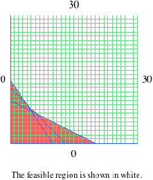
For the current solution x=(5,15/2,0,0) the inequality is not satisfied: 25/2≱13, hence the cut is valid and it tightens the formulation. We can see this also graphically in Figure 2.
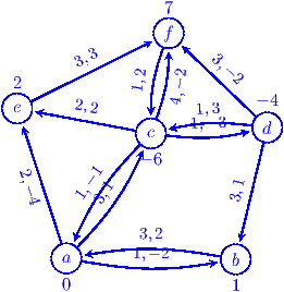
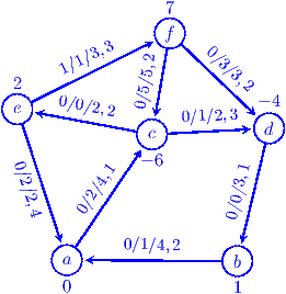
Consider the network N=(V,A,l≡ 0,u,b,c) of Figure 3 and let x* be the flow there represented.
\tikzset{ node/.style={circle,draw,fill=none,thick,minimum size=20pt,inner sep=0pt}, nondirectional/.style={very thick,black}, unidirectional/.style={nondirectional,shorten >=2pt,-stealth}, bidirectional/.style={unidirectional,bend right=10}, weight/.style={sloped,font=\small} } \begin{tikzpicture}[scale=8] \node [node] (a) at (-0.956460, -0.365955) {$a$}; \node at (a) [below=9pt] {$0$}; \node [node] (b) at (-0.462372, -0.368572) {$b$}; \node at (b) [below=9pt] {$1$}; \node [node] (c) at (-0.709751, -0.002069) {$c$}; \node at (c) [below=9pt] {$-6$}; \node [node] (d) at (-0.370297, 0.015660) {$d$}; \node at (d) [above=9pt] {$-4$}; \node [node] (e) at (-1.100000, 0.070901) {$e$}; \node at (e) [above=9pt] {$2$}; \node [node] (f) at (-0.657976, 0.290306) {$f$}; \node at (f) [above=9pt] {$7$}; \path [unidirectional] (a) edge node[weight,above=0pt,pos=0.5] {$0/3/4,1$} (c); \path [unidirectional] (b) edge node[weight,above=0pt,pos=0.5] {$0/1/4,2$} (a); \path [unidirectional] (c) edge node[weight,above=0pt,pos=0.5] {$0/1/2,3$} (d); \path [unidirectional] (c) edge node[weight,above=0pt,pos=0.5] {$0/0/2,2$} (e); \path [unidirectional] (d) edge node[weight,above=0pt,pos=0.5] {$0/0/3,1$} (b); \path [unidirectional] (e) edge node[weight,below=0pt,pos=0.5] {$0/2/2,4$} (a); % to use for bidirectional arcs % \path [bidirectional] (e) edge node[weight,below=0pt,pos=0.5] {$3/ /4,4$} (a); % \path [bidirectional] (a) edge node[weight,below=0pt,pos=0.5] {$3/ /4,4$} (e); \path [unidirectional] (e) edge node[weight,above=0pt,pos=0.5] {$0/0/3,3$} (f); \path [unidirectional] (f) edge node[weight,above=0pt,pos=0.5] {$0/4/5,2$} (c); \path [unidirectional] (f) edge node[weight,above=0pt,pos=0.5] {$0/3/3,2$} (d); \end{tikzpicture
Argue that the flow x* is feasible and give its cost.
Solution
The flow is feasible because:
Its cost is 30.
Draw the residual network N(x*) explaining briefly how you find the capacity on the arcs of N(x*) (it suffices to show a couple of examples).
Solution
Example:
|
Argue that x* is a minimum cost cycle for N.
Solution
There is no negative cost cycle in the residual network, hence for the
min cost optimality theorem the flow is optimal.
Suppose now that the lower bound to the flow in the arc ef is set to 1 while all the rest remains unchanged, thus yielding the network N′=(V,A,l′,u,b,c). Find a new feasible flow and explain how you found it.
Solution
To find a feasible flow we need to transform the network removing
lower bounds on arcs. This is done as seen in class by decreasing the
balance value of tail node by 1 and increasing the one of the head
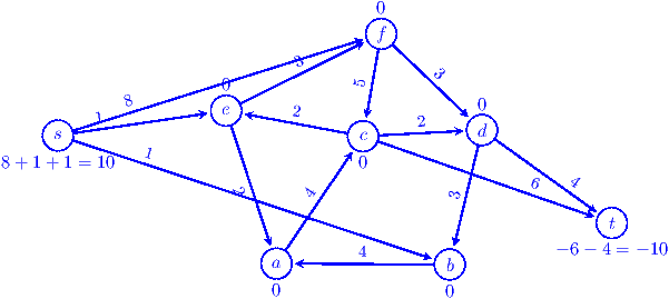
node by the same amount. We then construct an st network as shown in
Figure 4.
This is an instance of max flow that we solve by augmenting path algorithm (Ford-Fulkerson). We find:
sfdt 3
sfcdt 1
sfct 4
seact 1
sbact 1
The flow saturates the source arcs hence it is a feasible flow.
Find an optimal cost flow x′ for N′.
Solution
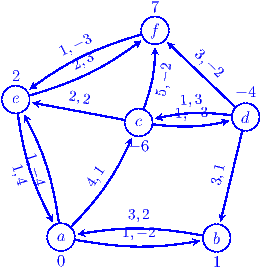
From the previous task the feasible flow is represented in
Figure 5. We obtain it going backwards in the
transformations applied earlier. (In specific, we reintroduced the
lower bound and hence established xef=1.) In the same figure
right the residual network in which there are no negative cost cycles.
It occurs that the new flow is obtained by augmenting the previous one through a zero cost cycle fcaef in the residual network N(x*). Hence the cost of the flow remains the same and there continue not to be improving cycles, hence it is optimal.
Decompose x′ into path and cycle flows and explain how you found each single component in the decomposition.
Solution
We apply DFS from any vertex with b(v)>0 and finish the path in a
vertex with b(v)<0 or in a cycle.
The decomposition yields only paths:
fc 5
fd 3
ba 1
ac 1
eacd 1
ef 1
The Danish Research Council has to decide which research projects to finance. The total budget for the projects is 20 million Dkk. The table below shows the evaluation from 0 (worst) to 2 (best) that the projects received by the external reviewers and the amount of money required.
1 2 3 4 5 Evaluation score 1 1.8 1.4 0.6 1.4 Investment (in million of DKK) 6 12 10 4 8
Projects 2 and 3 have the same coordinator and the Council decided to grant only one of the two.
The Council wants to select the combination of projects that will maximize the total relevance of the projects, that is, the sum of the evaluation score while remaining within the budget.
Formulate the problem of deciding on which project the Council has to invest as an integer linear programming problem P.
Solution
In .lp format:
| }\* Problem: lp3 *\ Maximize tot: + x(1) + 1.8 x(2) + 1.4 x(3) + 0.6 x(4) + 1.4 x(5) Subject To budget: + 6 x(1) + 12 x(2) + 10 x(3) + 4 x(4) + 8 x(5) <= 20 a: + x(2) + x(3) <= 1 Bounds 0 <= x(1) <= 1 0 <= x(2) <= 1 0 <= x(3) <= 1 0 <= x(4) <= 1 0 <= x(5) <= 1 End |
We want the IP instance solved using the branch-and-bound
algorithm. What is the optimal solution x* to the LP relaxation
P′? [Hint: use glpsol to find out. You find a skeleton with
the input data in the online version of this document.]
| set P; param score{P}; param crone{P}; param B; # # Your model here # solve; display something; data; set P := 1 2 3 4 5; param : score crone := 1 1 6 2 1.8 12 3 1.4 10 4 0.6 4 5 1.4 8; param B := 20; end; # in case you need data transposed: # 1 1.8 1.4 0.6 1.4 # 6 12 10 4 8 |
Solution
The following glpk model gives solution x→=[1,0.5,0,0,1] and
z=3.3.
| set P; param score{P}; param crone{P}; param B; var x{i in P} >=0, <=1; maximize tot: sum{i in P} score[i]*x[i]; subject to budget: sum{i in P} crone[i]*x[i] <= B; a: x[2]+x[3]<=1; # b: x[2]<=0; # c: x[5]<=0; # c: x[3]>=1; solve; display tot; display x; data; set P := 1 2 3 4 5; param : score crone := 1 1 6 2 1.8 12 3 1.4 10 4 0.6 4 5 1.4 8; param B := 20; end; |
The rounding heuristic applied to the solution x* gives a feasible solution x′. Which one? With the knowledge collected until this stage which of the three following statements is correct:
(Remember to justify your answer.)
Solution
The rounding heuristic updates x* setting x2=0 or x2=1. The
latter gives an infeasible solution while the former gives [1,0,0,0,1]
with value 2.4. We cannot say at this stage if x′ is optimal because
the optimality gap 3.3–2.4 is not closed. Hence (iii) is correct.
The two subproblems generated by the branch-and-bound algorithm after finding x* correspond to choosing or not choosing a particular project. Which one?
Solution
The solution is [1,0.5,0,0,1] and the only fractional variable is
x2 hence we branch on it.
Suppose the branch-and-bound algorithm considers first the subproblem corresponding to not choosing this project. Let’s call this subproblem and its corresponding node in the search tree SP1. What is the optimal solution to its LP relaxation?
Solution
Adding the constraint x2<=0 to the GLPK code above we obtain:
| x=[1, 0, 0.2, 1,1] |
and z=3.3.
Next, the branch-and-bound algorithm considers the subproblem corresponding to choosing the project, i.e., subproblem SP2. Find the optimal solution to its LP relaxation. Which are the active nodes (i.e., open subproblems) at this point?
Solution
Adding the constraint x2>=1 to the GLPK code above we obtain:
| x=[0, 1, 0, 0, 1] |
and z=3.2. This is an integer solution and hence a lower bound.
Node SP2 is not active since an integer solution prunes the subtree. The other node SP1 has however still potential to find a better solution since its upper bound is 3.3>3.2, hence the list of active nodes contains SP1.
How does the branch and bound end?
Solution
We need to examine the active nodes. Hence we branch once more with
x3≤ 0 (subproblem SP3) and x3≥ 1 (subproblem SP4). The LP
relaxation of SP3 gives an integer solution [1,0,0,1,1] of value 3 and
SP4 gives [0.33,0,1,0,1] of value 3.13. Hence the upper bound from
subtree SP1 is 3.13 which is smaller than the lower bound 3.2 of SP2 and
we can prune SP4 by bounding. The optimal solution is the one on node
SP2.
Some video camera must be allocated to watch the corridors of a museum. The graphs in Figure 6 represent the two floors of the museum, in which arcs correspond to corridors and vertices to the crossing points between corridors. A camera, allocated on a vertex, is able to watch all and only the arcs incident to the vertex. The problem in each floor consists in determining the minimal number of cameras and their position in order to watch all the corridors.
\tikzstyle{vertex}=[circle,draw,fill=none,thick,minimum size=12pt,inner sep=0pt,font=\scriptsize] \tikzstyle{selected vertex} = [vertex, fill=red!24] \tikzstyle{edge} = [draw,thick,-] \tikzstyle{arc} = [draw,thick,->,shorten >=1pt,>=stealth'] \tikzstyle{arcl} = [draw,thick,->,shorten >=1pt,>=stealth',bend left=25] \tikzstyle{arcr} = [draw,thick,->,shorten >=1pt,>=stealth'] \tikzstyle{weight} = [font=\small] \tikzstyle{selected edge} = [draw,line width=5pt,-,red!50] \tikzstyle{ignored edge} = [draw,line width=5pt,-,black!20] \begin{tikzpicture}[scale=0.9, auto,swap] % First we draw the vertices \foreach \pos/\name/\bv in {{(0,0)/8/ }, {(2,0)/9/ }, {(4,0)/10/ }, {(6,0)/11/ }, {(0,1)/4/ }, {(2,1)/5/ }, {(4,1)/6/ }, {(6,1)/7/ }, {(2,2)/1/ }, {(4,2)/2/ }, {(6,2)/3/ }}{ \node[vertex] (\name) at \pos {$\name$}; \node at \pos [below=9pt] {\bv}; } % Connect vertices with edges and draw weights - Forward arcs \foreach \source/\dest/\weight in { 8/9/{ }, 9/10/{ }, 10/11/{ }, 11/7/{ }, 7/6/{ }, 6/5/{ }, 5/4/{ }, 4/8/{ }, 5/1/{ }, 6/2/{ }, 5/9/{ }, 2/3/{ }, 7/3/{ } }{ \path[edge] (\source) -- node[weight] {$\weight$} (\dest); } \end{tikzpicture} % \hspace{2cm} \begin{tikzpicture}[scale=0.9, auto,swap] % First we draw the vertices \foreach \pos/\name/\bv in {{(0,0)/8/ }, {(2,0)/9/ }, {(6,0)/10/ }, {(0,1)/4/ }, {(2,1)/5/ }, {(4,1)/6/ }, {(6,1)/7/ }, {(2,2)/1/ }, {(4,2)/2/ }, {(6,2)/3/ }}{ \node[vertex] (\name) at \pos {$\name$}; \node at \pos [below=9pt] {\bv}; } % Connect vertices with edges and draw weights - Forward arcs \foreach \source/\dest/\weight in { 8/9/{ }, 9/10/{ }, 10/7/{ }, 7/6/{ }, 6/5/{ }, 5/4/{ }, 4/8/{ }, 5/1/{ }, 6/2/{ }, 5/9/{ }, 2/3/{ }, 7/3/{ } }{ \path[edge] (\source) -- node[weight] {$\weight$} (\dest); } \end{tikzpicture
Figure 6: Two graphs representing the two floors of the museum of Task 4. On the left the first floor, on the right the second floor. [You find online the code of these graphs exhibiting the list of edges.]
Formulate the problem
in terms of integer linear programming.
Solution
The problem is a vertex covering problem. The formulation that we saw in class is the following:
|
A weak dual of the vertex covering problem is the maximum matching problem.
What can you say about the possibility to solve the problems on the two floors using only linear programming? (Remember to justify your answers.)
Solution
In one of the exercises during the course whose answer can also be found in [B1] we saw that in the general case the vertex covering has fractional solutions. However the constraint matrix has only two entries different from zero in each column. We saw that such a matrix for undirected graphs is TUM if it is the incident matrix of a bipartite graph. A bipartite graph can be identified by the fact that it has no odd cycles. The graph on the left has no odd cycle, and it is indeed a bipartite graph with vertex partition (1,3,4,6,9,11) and (8,5,7,10,2). The solution to the vertex cover will be integer. The graph on the right instead has an odd cycle hence it is not bipartite and we have no element to rule out the possibility of fractional solutions. Solving the problem however will give an integer solution.
x[1].val = 0
x[2].val = 1
x[3].val = 0
x[4].val = 0
x[5].val = 1
x[6].val = 0
x[7].val = 1
x[8].val = 1
x[9].val = 0
x[10].val = 1
x[11].val = 0
x[1].val = 0
x[2].val = 1
x[3].val = 0
x[4].val = 0
x[5].val = 1
x[6].val = 0
x[7].val = 1
x[8].val = 1
x[9].val = 1
x[10].val = 0
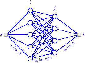
While your are holding this exam, the staff at IMADA will take a final decision about the creation of a new study area for students in the Mathematical Library. If the decision is positive some journals currently stored in the library will have to be moved in secondary facilities such as the basement or at the central Library. Each secondary storage facility has limited capacity and a particular access cost for retrieving information. Through appropriate data collection, made available by the diligent work of Tove, we can determine the usage rates for the information needs of the users. Let bj denote the capacity storage of facility j and vj denote the access cost per unit item from this facility. In addition, let ai denote the number of items of a particular class i requiring storage and let ui denote the expected rate (per unit of time) that we will need to retrieve books from this class. Our goal is to help Tove in deciding where to store the journals in a way that will minimize the expected retrieval cost.
Show how to formulate the problem of determining an optimal policy as a network flow problem;
Describe briefly an algorithm and explain the computational cost of its operations (only stating the total computational complexity without explanation is not enough).
Solution
The problem is a transportation problem with data represented in Figure 7.
The problem can be solved by a min cost flow algorithm such as the cycle canceling algorithm. One first has to find a feasible flow, by solving a max flow problem. The flow has to saturate all source outgoing arcs. Then the flow is augmented through cycles of negative cost in the reduced network. It turns out, however, (Evans, 1984) that the following greedy algorithm is optimal: repeatedly assign items with the greatest retrieval rate to the storage facility with lowest access cost.
Consider the following LP problem [you find online its data in text format]:
| |||||||||||||||||||||||||||||||||||||||||||||||||||||||||
and call x5,x6 the two slack variables to bring the problem in standard form.
Using only matrix computations, like in the revised simplex method,
calculate the value of the variables corresponding to a solution x*
with xB*=(x2, x3) basic variables and xN*=(x1,x4,x5,x6) non
basic variables. [Hint to be faster in inverting the matrix AB you
can use any program for linear algebra. For example, in R, the inverse
of a matrix can be calculated by solve and matrix
multiplications by %*%.]
Solution
From the theory we know that xB=AB−1b. The matrices AB for
xB=(x2, x3) and AN for xB=(x1, x4, x5, x6) are:
| AB= |
| AN= |
|
and its inverse computed in R with:
A=matrix(c(2,1,3,2),ncol=2,byrow=FALSE)
A1=solve(A)
A1%*%A # let's check
is
| AB−1= |
|
Thus:
b=c(5,3)
A1%*%b
     [,1]
[1,]  1
[2,]  1
which gives x2=1, x3=1.
Show that the solution found at the previous subtask is optimal but that it is not unique. Consequently, express all optimal solutions.
Solution
To check whether this solution is optimal we need to compute the reduced
costs cN of the non basic variables. From theory we need two calculations:
Hence in R:
cN=c(2,3,0,0)
cB=c(3,5)
AN=matrix(c(1,1,1,3,1,0,0,1),ncol=4,byrow=FALSE)
y=cB%*%A1
cN-y%*%AN
    [,1] [,2] [,3] [,4]
[1,]    0  -1   -1   -1
Since all reduced costs are non-positive the solution is optimal. However one reduced cost is null. This is an indication that there are infinite optimal solutions. To find them we need to make a linear combination of the optimal vertices. Let’s bring x1 in basis. To decide which variable between x2 and x3 is going to leave the basis we need to compute how much we can increase them:
| x′B=xB−AB−1ANxN x′B=xB−AB−1at≥ 0 |
where a is the column of the variable entering in the basis.
> a=c(1,1)
> A1%*%a
     [,1]
[1,]   -1
[2,]    1
| x′B= |
| − |
| t≥ 0 ⇒ |
|
Hence the variable to leave the basis is x3. The new AB matrix is:
| AB= |
|
and its inverse computed in R with:
> AB=matrix(c(2,1,1,1),ncol=2,byrow=FALSE)
> AB
     [,1] [,2]
[1,]    2    1
[2,]    1    1
> AB1=solve(AB)
> AB1
     [,1] [,2]
[1,]    1   -1
[2,]   -1    2
is
| AB−1= |
|
Thus:
b=c(5,3)
AB1%*%b
     [,1]
[1,]  2
[2,]  1
which gives x2=2, x1=1.
All the solutions can be expressed by linear combination of the two solutions found: α x→*+(1−α) x→′, α≥ 0, that is,
|
Which minimal change in the data of the problem, maintaining all data integer, would make x* become the unique optimal solution.
Solution
Changing the cost coefficient of x1 in the objective function from 2
to 1 would ensure that all reduced cost become negative and would not
affect the feasibility of x*, hence it would become the only optimal
solution.
Suppose we wish to consider a change in the right-hand side term of the second constraint, adding a value є ∈ ℝ.
Solution
From the matrix representation of the simplex method we have
b=A−1b and z=yTb. Hence,
| b=A−1b= |
|
| = |
| ⇒ |
| ⇒ |
|
Hence for є ∈ [−1/2,1/3] the solution x* remains feasible. Since in this case changing the b terms does not affect the reduced costs, then all previous optimal solutions remain optimal in that interval. The objective value can be calculated using the multipliers (here y). Hence:
|
| =5+3+є=8+є |