| DM841 (E23) - | Heuristics and Constraint Programming for |
| Discrete Optimization |
Obligatory Assignment 5
Preamble
-
This is the second of two assignments on discrete optimization that will be used to determine your final grade. The assignment will be graded with internal censorship. The final grade for the course will be an overall assessment of the two graded assignments starting from the arithmetic average.
-
Deadline: January 15, 2024, at 12:00
-
The assignment has to be carried out individually. Communication for feedback and inspiration with peers is allowed but it should be kept to a minimum. In case, you are welcome to ask to the teacher via the Disqus post.
-
You have to submit:
-
a PDF document containing max 10 pages of description of the heuristic algorithms you have designed and implemented and the results you have obtained on the data sets available.
-
source code of your implementations in python
-
-
The submission procedure is via git.imada.sdu.dk as for the other assignments in this course (see Assignment 1 for details). The structure of your repository is listed below:
    Repo_march
    |-	asg5
    │  	├── data
    │   │   ├── dir1
    │  	│   └── dir2
    │  	├── src
    │  	└── tex
    └────── README.md
- The report must be in pdf format inside
doc.
Capacited Vehicle Routing
In vehicle routing problems we are given a set of transportation requests and a fleet of vehicles and we seek to determine a set of vehicle routes to perform all (or some) transportation requests with the given vehicle fleet at minimum cost; in particular, we decide which vehicle handles which requests in which sequence so that all vehicle routes can be feasibly executed.
The capacitated vehicle routing problem (CVRP) is the most studied version of vehicle routing problems.
In the CVRP, the transportation requests consist of the distribution of goods from a single depot, denoted as point $0$, to a given set of $n$ other points, typically referred to as customers, $N=\{1,2,\ldots,n\}$. The amount that has to be delivered to customer $i\in N$ is the customer’s demand, which is given by a scalar $q_i\geq 0$, e.g., the weight of the goods to deliver. The fleet $K=\{1,2,\ldots,|K|\}$ is assumed to be homogeneous, meaning that $|K|$ vehicles are available at the depot, all have the same capacity $Q>0$, and are operating at identical costs. A vehicle that services a customer subset $S\subseteq N$ starts at the depot, moves once to each of the customers in $S$, and finally returns to the depot. A vehicle moving from $i$ to $j$ incurs the travel cost $c_{ij}$.
The given information can be structured using an undirected graph. Let $V=\{0\}\cup N=\{0,1,\ldots,n\}$ be the set of vertices (or nodes). It is convenient to define $q_0:=0$ for the depot. In the symmetric case, when the cost for moving between $i$ and $j$ does not depend on the direction, i.e., either from $i$ to $j$ or from $j$ to $i$, the underlying graph $G=(V,E)$ is complete and undirected with edge set $E=\{e=(i,j)=(j,i) : i,j\in V,i\neq j\}$ and edge costs $c_{ij}$ for $\{i,j\} \in E$. Overall, a CVRP instance is uniquely defined by a complete weighted graph $G=(V,E,c_{ij},q_i)$ together with the size $|K|$ of the of the vehicle fleet $K$ and the vehicle capacity $Q$.
A route (or tour) is a sequence $r=(i_0,i_1,i_2,\ldots,i_s,i_{s+1})$ with $i_0=i_{s+1}=0$, in which the set $S=\{i_1,\ldots,i_s\}\subseteq N$ of customers is visited. The route $r$ has cost $c(r)=\sum_{p=0}^sc_{i_p,i_{p+1}}$. It is feasible if the capacity constraint $q(S):=\sum_{i\in S}q_i\leq Q$ holds and no customer is visited more than once, i.e., $i_j\neq i_k$ for all $1\leq j\leq k\leq s$. In this case, one says that $S\subseteq N$ is a feasible cluster. A solution to a CVRP consists of $K$ feasible routes, one for each vehicle $k\in K$. The routes $r_1,r_2,\ldots,r_{|K|}$ and the corresponding clusters $S_1,S_2,\ldots,S_{|K|}$ provide a feasible solution to the CVRP if all routes are feasible and the clusters form a partition of $N$. Hence, the CVRP consists of two interdependent tasks:
(i) the partitioning of the customer set $N$ into feasible clusters $S_1,\ldots,S_{|K|}$;
(ii) the routing of each vehicle $k\in K$ through $\{0\}\cup S_k$.
At the DIMACS Implementation Challenge on Vehicle Routing seven other variants of vehicle routing problems are presented. You can choose to focus on one of those if you wish. The higher the the problem is in the numbered list, the more challenging the solution becomes but also the more rewarding could be the grade.
In the following sections and in the git repository you find instances, starting code and details for the Capacitated Vehicle Routing Problem (CVRP) only. If you choose to solve other variants of VRP you might still reuse some of the code provided for your purposes but you will need to adapt it to your case. Anyway, you are not obliged to use the code provided. In choosing test instances for other VRP variants, avoid instances with ceiling or flooring effects in the comparison of algorithms.
The section “Your Tasks” remains valid for all variants.
Starting Package
Pulling your git repository for this course you will find a directory data/ containing the instances,
a directory src/ containing some initial Python 3 code to read the
instances, output a solution and produce a graphical view of solutions.
The code also provides the same framework as in Assignment 4 to organize your
implementation.
Instances
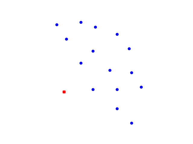
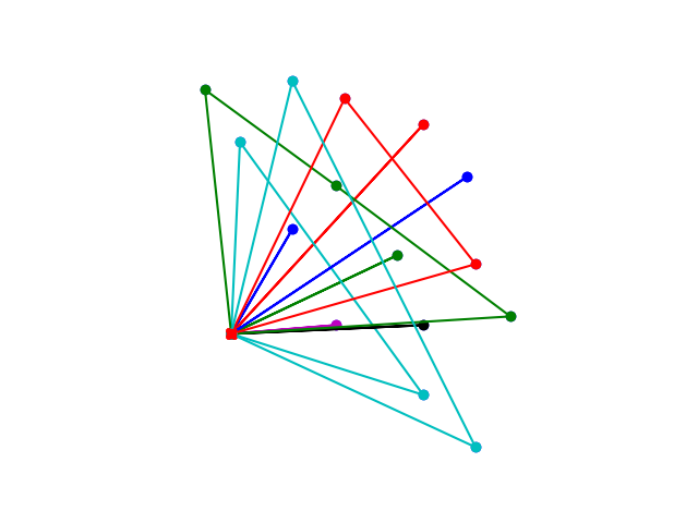
In the directory data/ you find the instance P-n016-k08.xml that is a
small toy instance with 16 nodes. This instance and a heuristic solution
is represented in the figure.
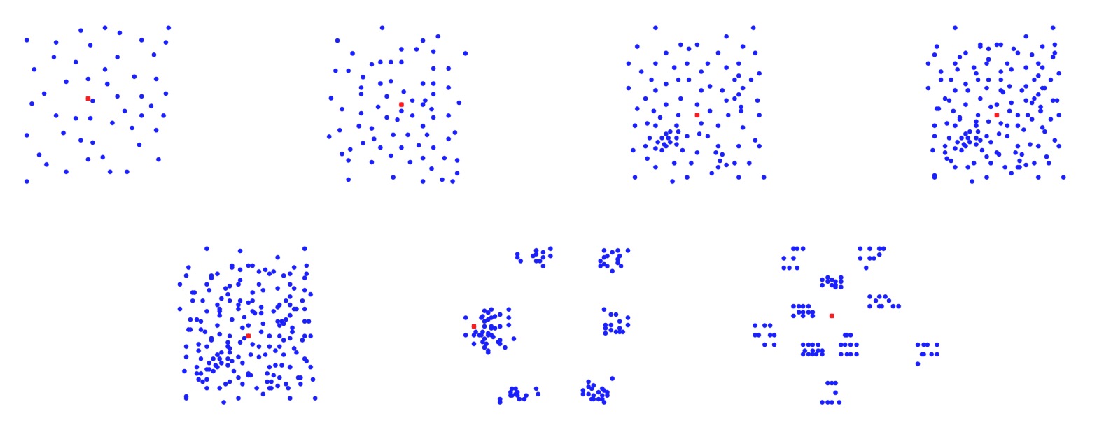
In the directory data/CMT you find the set CMT[^1] of middle size
instances with number of nodes ranging between 51 and 200, and in the
directory data/Golden you find the set Golden[^2] of large size
instances with number of nodes ranging between 241 and 484. The
displacement of the nodes in these two classes of instances is depicted in the
following two figures.

The best known solutions for these instances are reported in the table. A star indicates that the solution has been proven optimal.
| instance | nodes | best known |
|---|---|---|
| CMT01 | 51 | 524.61* |
| CMT02 | 76 | 835.26* |
| CMT03 | 101 | 826.14* |
| CMT04 | 151 | 1028.42* |
| CMT05 | 200 | 1291.29* |
| CMT11 | 121 | 1042.11* |
| CMT12 | 101 | 819.56* |
| instance | nodes | best known |
|---|---|---|
| Golden_01 | 241 | 5623.47 |
| Golden_02 | 321 | 8404.61 |
| Golden_03 | 401 | 11036.22 |
| Golden_04 | 481 | 13592.88 |
| Golden_05 | 201 | 6460.98 |
| Golden_06 | 281 | 8404.26 |
| Golden_07 | 361 | 10102.68 |
| Golden_08 | 441 | 11635.34 |
| Golden_09 | 256 | 579.71 |
| Golden_10 | 324 | 736.26 |
| Golden_11 | 400 | 912.84 |
| Golden_12 | 484 | 1102.69 |
| Golden_13 | 253 | 857.19 |
| Golden_14 | 321 | 1080.55 |
| Golden_15 | 397 | 1337.92 |
| Golden_16 | 481 | 1612.50 |
| Golden_17 | 241 | 707.76 |
| Golden_18 | 301 | 995.13 |
| Golden_19 | 361 | 1365.60 |
| Golden_20 | 421 | 1818.32 |
In addition, you also find the Augerat instances.
Source Code
The Python code in the directory src/ contains the following files:
-
problem.pythat implements the classProblemto maintain the data associated with the input instance. It contains an instance reader for the XML format. Objects of this class contain the following data that will be relevant to you:capacitygiving the capacity of the vehicle andnodesthat is a tuple container of the nodes of the given network. Each element from the tuplenodesis a dictionary with the following keys and values:id, the original identifier of the node from the input file,pt, the coordinates of the node in complex numbers notation as we saw for the TSP,tp, the type of customer: 0 if a depot and 1 if a customer,rq, the quantity demanded by the node (if it is a depot this value is 0). Nodes in the tuplenodesare organized in such a way that the depot is the first element followed by all others. Each node can be accessed in constant time through the index in the tuple. Hence, internally the depot has always index zero while in the instance file it might be any identifier.The class
Problemcontains also methods for printing the instance, reporting statistics, calculating distances and plotting. -
solution.pythat implements the classSolutionto store data relative to a candidate solution.The class
Solutioncontains also methods for writing the solution file and for plotting the solution. These latter methods assume that solutions are represented as lists of lists, where every inner list representing a route starts with the depot and ends with the depot. Note that the solution writer must output the original identifier of the nodes and not the one used to represent them internally. -
main.pythat implements the main program defining the objects and calling the methods defined in the other files. It provides a starting example that can be modified at your best convenience. It also defines the parameters to be specified when the program is run. -
api/*contains the implementation of some of the heuristic methods seen in the course. It is possible to modify this part as well.
The program is executed as specified below:
$ python3 main.py --budget 120 --seed 1 --log-level info --output-file instance.sol \
    --plot-file P-n016-k08_sol.png ../data/P-n016-k08.xml
It is possible to modify all these files and to add new ones. For example, you may want to add a Makefile program as seen in Assignment 4.
Finally, make sure to specify how to call your program in the file README.md.
Your Tasks
-
Design and implement one or more construction heuristics.
-
Design and implement one or more iterative improvement algorithms. They must terminate in a local optimum.
-
Design and implement metaheuristic algorithms. They can use as components the elements from points 1. and 2. used either as black boxes or modified according to the metheuristic principles.
-
Undertake an experimental analysis where you compare the algorithms from points 1. and 2. and configure the algorithms from point 3. to perform best on average on instances of the largest type. Overall never exceed one minute of running time for a single run of an algorithm.
-
Describe the work done in a report of at most 10 pages. The report must at least contain a description of the best algorithm designed and the experimental analysis conducted. The level of detail must be such that it makes it possible for the reader to reproduce your work.
The report must present:
- the modeling decisions:
- solution components and construction rules
- local search compoenents,
- a sketch of the algorithm developed
- the implementation decisions:
- delta evaluation
- neighborhood search
- computational costs of the step in local search or the construction rule
- the best results on the given instances in a table.
- the modeling decisions:
-
Submit your work making sure that the code provided will execute the best algorithm with a time limit of one minute when run from command line as follows:
$ python3 main.py --budget 60 --seed 1 --log-level info --output-file instance.sol ../data/instance.xml
and reports in instance.sol the best solution found in the format
explained below. The parameters --seed and --budget are for the random seed
and the overall time limit in seconds, respectively. The program must solve the specified instance and halt before the specified time limit.
Remarks
Remark 1 Make sure and give evidence that the results obtained by the algorithms in the point 3. above are better then those obtained in point 1. and 2.
Remark 2 The metaheuristics designed in point 3. can be any among those encountered in the lectures. More specifically, you can choose one or more algorithm templates among those from the groups treated in class:
- local search based metaheuristics
- construction based metaheuristics
- population based metaheuristics
A few, well thought algorithms are better than many naive ones. However, it is expected that you compare a few alternatives.
Remark 3 You should be able to indicate in your report the name of the metahuristic(s) implemented. If your algorithm differ in some elements from the standard templates of the metaheuristics seen in class you must state that in the report and if it is an original attempt you should try to indicate which approach seen in class gets closer to it.
Remark 4 This is a list of factors that will be taken into account in the evaluation (possibly in order of importance):
- correctness of results claimed after running the submitted program
- quality of the final results;
- level of detail of the study;
- complexity and originality of the approaches chosen;
- presence of the analysis of the computational costs involved in the main operations of the local search.
- organization of experiments that guarantees reproducibility of conclusions;
- clarity of the report;
- effective use of graphics in the presentation of experimental results.
- correctness in the classification of the algorithms, that is, using the right names for the metaheuristics described
Output Format
At termination your program must write the solution in the format described below in a file.
The starting code provided expects you to implement this in the function Solution.output.
The function is called from the main file.
The solution file must list the routes one per line. Each route is a comma separated list of nodes to be visited in the given order. The node identifier must be the original one from the input file. Routes must start with the depot and finish with the depot.
The following listing provides an example of solution file for a valid solution to the instance CMT02:
    76,1,2,3,4,5,6,7,76
    76,8,9,10,11,12,13,76
    76,14,15,16,17,18,19,20,76
    76,21,22,23,24,25,26,27,76
    76,28,29,30,31,32,76
    76,33,34,35,36,37,38,39,76
    76,40,41,42,43,44,45,76
    76,46,47,48,49,50,51,52,76
    76,53,54,55,56,57,58,59,76
    76,60,61,62,63,64,65,66,76
    76,67,68,69,70,71,72,73,74,75,76
Solutions files have extension .sol.
The submission system will execute your program and compare the results against your peers’ones on a set of unspecified instances. Therefore, you should submit your best algorithm early and eventually revise your submission. Before submitting, test your implementation on the IMADA virtual computer lab. If you are using additional python modules not present in setting of the Computer Lab machines, write this in the README.md file and in an additional file requirements.txt.