Basis vectors
Contents
5. Find another basis for R^5
%lets just take a set of vectors
V = randi([0,10],5)

%If the rank is 5, this is a basis
rank(V)
V =
     8     6     5     4    10
     0     2     2     4     8
    10     5     5    10     1
     8    10     6     0     2
     5     6     7     9     3
ans =
     5
Now find the vector w in the new basis
w = [1;2;3;4;5]

c = V\w
w =
     1
     2
     3
     4
     5
c =
   -0.4686
    0.9841
   -0.3015
    0.4415
   -0.1414
Check
V*c
ans =
    1.0000
    2.0000
    3.0000
    4.0000
    5.0000
6. Orthonormal basis
1. Find a non-standard orthonormal basis for R^2 and R^3 Use the Gram-Schmidt Process
%first, a random set of vectors
V = randi([0,10],2)

%Take the first one and normalize
v1 = V(:,1);
e1 = v1 / sqrt(v1'*v1)
%The norm is now 1
e1'*e1
V =
     7     7
     1     1
e1 =
    0.9899
    0.1414
ans =
    1.0000
%Take the second vector and make it orthogonal
v2 = V(:,2);
c = v2'*e1;
v = v2 - c*e1
%check
v'*e1
v =
   1.0e-15 *
    0.8882
    0.1110
ans =
   8.9495e-16
And normalize
e2 = v / sqrt(v'*v)
%The norm is now 1
e2'*e2
e2 =
    0.9923
    0.1240
ans =
    1.0000
The basis is then
[e1,e2]
ans =
    0.9899    0.9923
    0.1414    0.1240
The same for R^3
%first, a random set of vectors
V = randi([0,10],3)

for i = 1:3  %cycle trough the vectors
    v = V(:,i);
    for j = 1:(i-1)  %go through all the previous vectors
        c = v'*e(:,j);
        v = v - c*e(:,j);
    end
    e(:,i) = v / sqrt(v'*v); % normalize
end

e
V =
     7     7     3
     5     9     7
     8     9     2
e =
    0.5959   -0.4222    0.6832
    0.4256    0.8874    0.1771
    0.6810   -0.1852   -0.7085
%For and R^n, as a function
%function [ e ] = GramSchmidt( V, N )
%%GRAMSCHMIDT
%    for i = 1:N  %cycle trough the vectors
%        v = V(:,i);
%        for j = 1:(i-1)  %go through all the previous vectors
%         c = v'*e(:,j);
%            v = v - c*e(:,j);
%        end
%        e(:,i) = v / sqrt(v'*v); % normalize
%    end
%end


N=4 ;
V = randi([0,10],N) ;
GramSchmidt(V,N)
ans =
         0    0.8943    0.4410    0.0764
    0.7493   -0.2615    0.5680   -0.2182
    0.4683    0.0601   -0.2674    0.8400
    0.4683    0.3582   -0.6414   -0.4909
7.
n = 100;
dx = 2*pi/n;
x = linspace(-pi,pi,n+1); x(n+1)=[];

% Functions cos(x) and sin(2x)
f1 = cos(x);
f2 = sin(2*x);

norm1 = sqrt( f1*f1'*dx )
norm2 = sqrt( f2*f2'*dx )

product = f1*f2'*dx
norm1 =
    1.7725
norm2 =
    1.7725
product =
  -2.5810e-16
How about sin(nx) and cos(nx)
n1=1; n2=2; n3=3; n4=4;
f1 = cos(n1*x);
f2 = sin(n2*x);
f3 = cos(n3*x);
f4 = sin(n4*x);

norm1 = sqrt( f1*f1'*dx )
norm2 = sqrt( f2*f2'*dx )
%always 1.7725
norm1 =
    1.7725
norm2 =
    1.7725
product1 = f1*f2'*dx
product2 = f1*f3'*dx
product3 = f2*f4'*dx
product1 =
  -2.5810e-16
product2 =
  -3.9064e-16
product3 =
   4.5342e-17
Functions cos(nx) and sin(nx) form a basis find the vector x^2 in this basis
%find coefficients for a given n:

N = 100;
dx = 2*pi/N;
x = linspace(-pi,pi,N+1); x(N+1)=[];

% Functions cos(nx) and sin(nx)
n=2;
b1 = cos(n*x);
b2 = sin(n*x);

%The function we are representing, x^2
f = x.*x;

%Coefficients cn = (f1,b1)/(b1,b1)
c1 =  (f*b1'*dx)  / ( b1*b1'*dx );
c2 =  (f*b2'*dx)  / ( b2*b2'*dx );
Find coefficients in the space of cos(nx) and sin(nx) for n<N-1
%function [ c1,c2 ] = Coefs( n )
%PRODUCT Summary of this function goes here
%  Detailed explanation goes here
%  for k = 1:n
%    N = 100;   dx = 2*pi/N;
%    x = linspace(-pi,pi,N+1); x(N+1)=[];
%
%    % Functions cos(nx) and sin(nx)
%    b1 = cos((k-1)*x);  b2 = sin((k-1)*x);
%    %The function we are representing, x^2
%    f = x.*x;
%
%    %Coefficients cn = (f1,b1)/(b1,b1)
%    c1(k) =  (f*b1'*dx)  / ( b1*b1'*dx ) ;
%    if k>1
%        c2(k) =  (f*b2'*dx)  / ( b2*b2'*dx );
%    else
%        c2(1) = 0; %sin(0x) = 0
%    end
%  end
%end

N=10;
[c1,c2] = Coefs(N)
c1 =
  Columns 1 through 7
    3.2905   -4.0013    1.0013   -0.4458    0.2513   -0.1613    0.1124
  Columns 8 through 10
   -0.0830    0.0638   -0.0507
c2 =
   1.0e-14 *
  Columns 1 through 7
         0    0.0107    0.0213   -0.0977    0.0711   -0.0817    0.1812
  Columns 8 through 10
   -0.1315    0.0284   -0.0462
Now lets check if we get the original vector
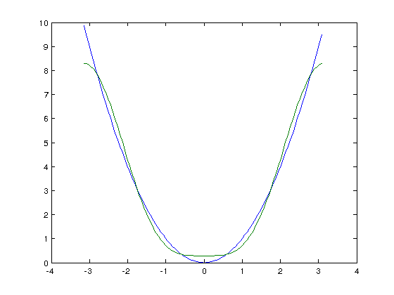
With N=3, we get an inaccurate result
k = 100;
N = 3;
dx = 2*pi/k;
x = linspace(-pi,pi,k+1); x(k+1)=[];

f=0*x;
for n = 1:N
    f = f + c1(n)*cos((n-1)*x);
    f = f + c2(n)*sin((n-1)*x);
end
plot(x,x.*x,x,f)
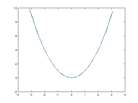
With N=10 it's much more accurate
k = 100;
N = 10;
dx = 2*pi/k;
x = linspace(-pi,pi,k+1); x(k+1)=[];

f=0*x;
for n = 1:N
    f = f + c1(n)*cos((n-1)*x);
    f = f + c2(n)*sin((n-1)*x);
end
plot(x,x.*x,x,f)