Session3

Exercise 2
Exercise 3
Exercise 4.

Exercise 2

Check doc nargin and doc nargout for details

%Define a function that can take up to 2 inputs and produce up to 2 outputs
% function [ sum, abssum ] = addme( a,b )
% ADDME
% %nargin is the number of arguments given. If 1, output is a+a. If 2,
% %output is a+b.
%  switch nargin
%    case 2
%        sum = a+b;
%    case 1
%        sum = a+a;
%    otherwise
%        sum = 0;
%  end
% %nargout is the number of output arguments requested. If it is 1, the only
% %thing that will be returned is sum. If it is > 1, both sum and absum will
% %be returned. It the second case we need to define abssum.
%  if nargout > 1
%    abssum = abs(sum);
%  end
%end

Exercise 3

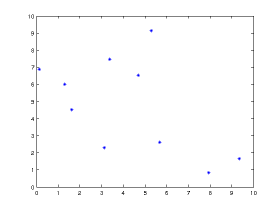
generate points

x = 10*rand(1,10)
y = 10*rand(1,10)

plot(x,y,'b*')

x =
  Columns 1 through 7
    9.3401    1.2991    5.6882    4.6939    0.1190    3.3712    1.6218
  Columns 8 through 10
    7.9428    3.1122    5.2853
y =
  Columns 1 through 7
    1.6565    6.0198    2.6297    6.5408    6.8921    7.4815    4.5054
  Columns 8 through 10
    0.8382    2.2898    9.1334

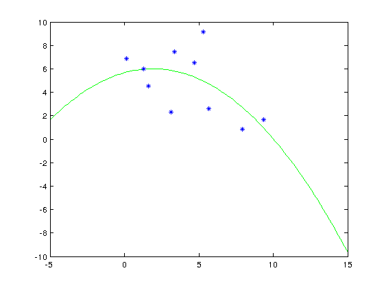
%Polyfit will fit a polynomial through the points:
p = polyfit(x,y,2);

Plot to check.

xfit = linspace(-5,15);
yfit = polyval(p,xfit);
plot(xfit,yfit,'g',x,y,'b*') %line is green ('g') and points are marked with blue stars ('b*')

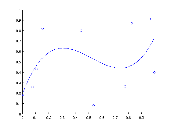
%The fit using fminsearch. fminsearch minimizes a function, so we need to
%define one. The function we need to minimize is the distance of the points
%from the polynomial.

% We want to find a polynomial of degree 3 that fits at best a given set of
% data.
% We start creating 10 points at random and plotting them:
data_points = rand(10,2);
scatter(data_points(:,1),data_points(:,2));
hold on

% Then, we set up a handler to a function that first calculates for each point the difference
% between the point measured and the point on a curve of order three and then calculates the sum
% of the squares of these discrepancies.
f = @(a) sum((data_points(:,2) - polyval(a,data_points(:,1))).^2);
% The polynomial that fits at best the data is the one that minimized the
% function square of errors given above. We have learnt to minimize
% functions with fminsearch:
[a,error] = fminsearch(f, [0, 0, 0, 0]);

% Now a contains the coefficient of the polynomial.
x = min(data_points(:,1)):0.01:max(data_points(:,1));
plot(x,polyval(a,x));
hold off

Exercise 4.

%vector as [x;y;z]
p0 = [0;0;1.5]; %starting point
u = [1;1;1];  %starting direction
ut = u / sqrt(u'*u); %normalized
g = [0;0;-9.81];
s = 10;
v0 = u*s ; % starting speed

%Landing time is
tl = (-v0(3) - sqrt(v0(3)^2 - 2*p0(3)*g(3)))/(g(3))

%location at landing time:
p = p0 + v0*tl + g*tl^2/2

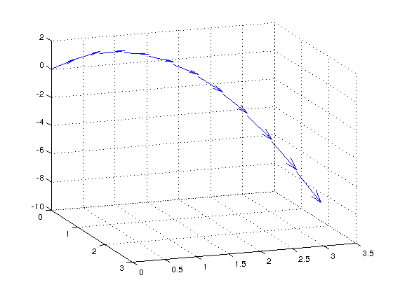
Vector fields Projectile Path Over Time using quiver3 \(\mathbf{p}(t)=\mathbf{v}t+\frac{\mathbf{a}t^2}{2}\)

\begin{align*} \begin{bmatrix}x\\y\\z \end{bmatrix} &=\begin{bmatrix}v_x\\v_y\\v_z \end{bmatrix} t+\frac{1}{2}\begin{bmatrix}a_x\\a_y\\a_z \end{bmatrix}t^2\\ &=\begin{bmatrix}2\\3\\10 \end{bmatrix} t+\frac{1}{2}\begin{bmatrix}0\\0\\-32 \end{bmatrix}t^2 \end{align*}

vz = 10; % velocity constant
a = -32; % acceleration constant
% Calculate z as the height as time varies from 0 to 1.
t = 0:.1:1;
z = vz*t + 1/2*a*t.^2;
% Calculate the position in the x-direction and y-direction.
vx = 2;
x = vx*t;
vy = 3;
y = vy*t;
% Compute the components of the velocity vectors and display the vectors
u = gradient(x);
v = gradient(y);
w = gradient(z);
scale = 0;

figure
quiver3(x,y,z,u,v,w,scale)
% Change the viewpoint of the axes to [70,18].
view([70,18])

Find the shooting angle to get the requested landing spot: aiming at [1,0,0]

% First define lower and upper limit for the initial direction
ulow = [0.001;0;1]; %I'm pretty sure it needs to be higher than this
uhigh = [100;0;1]; % and lower than this

% Normalize the direction vectors
ul = ulow/sqrt(ulow'*ulow);
uh = uhigh/sqrt(uhigh'*uhigh);

Get landingpoints for the high and low angels.

ll = landingpoint(p0,s*ul,0.1,0.1);
lh = landingpoint(p0,s*uh,0.1,0.1);
% Calculate the error (distance from the point we are aiming at)
% We are aiming at [1,0,0]
rl = ll(1)-1;
rh = lh(1)-1;

The landing point as a function:

%function [ p ] = landingpoint( p0,v0,c,k )
%  %LANDINGPOINT
%  g=[0;0;-9.81];
%  dt=0.001;
%  p=p0;v=v0;
%  while p(3) > 0
%    a = g - k*v -c * v*sqrt(v'*v);
%    pnew = p + v*dt;
%    vnew = v + a*dt;
%    p=pnew; v=vnew;
%  end
%  %In the end the solution bullet will be slightly underground,
%  %but it's accurate enough
%end

Now find the correct shooting angle. Lets use the bisection algorithm, one of the simplest algorithms for finding the zero of a function. We start knowing that there is a zero in the range [ulow,uhigh]. In this case the function is the error

delta = 10; %The error of the previous step
while delta > 0.001;
    % Define a new middle point between the too high and too low values
    umid = ulow+uhigh/2;
    um = umid/sqrt(umid'*umid); %Normalize
    lm = landingpoint(p0,s*um,0.1,0.1); % Find the landing point
    rm = lm(1)-1; % and the error for the middle point
    % Now if the lower and the middle point have different sign, there is a
    % zero between them. Continue to look for a zero between in the range
    % [ulow,umid].
    if rm*rl < 0
        uhigh = umid;
    % If not, we the zero must be in the range [umid,uhigh]
    else
        ulow = umid;
    end
    % Check the error, |rm|
    delta = sqrt(rm*rm);
end

Now the correct direction is umid.

um = umid/sqrt(umid'*umid) %Normalized
landingpoint(p0,s*um,0.1,0.1) %Check that it hits the desired position

Contents

Exercise 2

Exercise 3

Exercise 4.