Contents
Reading the data
We import the data from the data file.
clear; % it is good practice clearing the workspace at the beginning to avoid errors due to left over variables
A=xlsread('cars.xls') % we could have used also load("cars.txt")
A =
   335   717   586   340   104
   375   257   409   551   626
   491    43   614   292   445
   246   383   373   567   649
   554   600    18   250   177
Transition Matrix
Let's construct the matrix C from the matrix A. The sum of the values on each column must give 1 because every current car must be substituted with a new one (even of the same brand). To construct C we divide each element of the matrix by the sum over the rows.
s=sum(A,1); % a vector with an element for each column equal to the column-wise sum
C=A./repmat(s,[5,1]) % repmat replicates the vector 5 times in the first dimension
Note the array operation './' in the previous column as opposed to matrix division that is not defined in mathematics. The matrix C is the transition matrix. It is a stochastic matrix, that is, it has the property that the sum of its terms rowwis is 1.
C =
    0.1674    0.3585    0.2930    0.1700    0.0520
    0.1874    0.1285    0.2045    0.2755    0.3128
    0.2454    0.0215    0.3070    0.1460    0.2224
    0.1229    0.1915    0.1865    0.2835    0.3243
    0.2769    0.3000    0.0090    0.1250    0.0885
Deriving the distribution of cars in the periods
There are several ways to determine the distribution of cars in future periods. Here we use the array data strucutres for which Matlab is primarily implemented. You can print out intermidiate values to see understand what these lines do.
n = 5; % there are 5 brands
tmax = 10; % let's follow the market for 10 years
F = zeros(n,tmax);
p_0 = [426 436 364 437 336]; % the initial distribution of cars
F(:,1) = p_0/sum(p_0); % the initial car fractions
for t = 2:tmax
    F(:,t) = C * F(:,t-1);
end
We have thus computed the distribution throughout the periods.
Plot
We can now plot the distribution.
clrs='ygrmb'; % 5 colors, one for each brand
times = 1:tmax; % the x-axis

for k=1:n
    plot(times,F(k,:),'-ks','LineWidth',2,...
                       'MarkerEdgeColor','k',...
                       'MarkerFaceColor',clrs(k),...
                       'MarkerSize',8);
                   hold on
end
hold off
xlabel('time','FontSize',15);
ylabel('brand market share','FontSize',15);
set(gca,'FontSize',14)
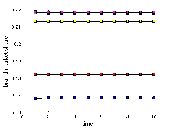
The result is quite peculiar, nothing seems to change. Is the result correct? Is it a special case or will it always be like that? You could try asking how things would change when we use different starting states. Try to generate different starting distributions of cars: F(:,1), for example with F(:,1)=[1 0 0 0 0]; or others at random. Try to do this and rerun the calculation to plot the new solutions. What do you observe?
Generating a random transition matrix
Another thing you could wonder is how things change if we keep the same starting state but we use a different transition matrix. We can generate a transition matrix at random but we must satisfy the constraint that in each column the sum of elements is 1.
clear; % let's clear the workspace from the previous values.
n=5;
C = zeros(n);
for k=1:n
    r = rand(n,1);
    r = r/sum(r);
    C(:,k)=r;
end
Each column of C consists of random numbers whose sum is one each run produces different random numbers and different results, unless the random number generator is initialized.
Steady state
If you have played with the changes suggested above, you may have observed that the plot reported above was a particular case. However, although the initial distribution may change and the distribution throughout the periods may also vary, what we observe is that in the long run the distrbution converges towards a stady distribution. We are interested in determining the steady state, that is, the state at which the application of a transition leads to the same state, ie, a vector x for which Ax=lambda x. This implies: (A-lambda I)x=0. The value lambda is said to be an eigenvalue and the state vector x an eigenvector. There are eigenvalues and eigenvectors only if (A-lambda I)x=0 has non trivial solution, ie, a solution different from the zero vector x=0. Theory on systems of linear equations shows that for this to happen the matrix (A-lambda I) must be singular, ie, det(A-lambda I)=0. This is equivalent to writing the characteristic polynomial and setting it equal to zero. The roots of the polynomial, ie, the solutions to the characteristic equation, are the eigenvalues. The corresponding eigenvectors can be derived consequently. In Matlab we find all eigenvalues and all eigenvectors as follows:
[V,D]=eig(C)
The eigenvalues lambda are reported on the diagonal of the matrix D. A theorem from linear algebra shows that if all the elements of the transition matrix are strictly positive (as in our case), then the process converges to a steady state that is the same for any initial state vector. Another theorem shows that if 1 is the dominant (largest) eigenvalue then the process converges towards a steady state expressed by the eigenvector that has eigenvalue 1. This means that for the eigenvector e1 with eigenvalue 1 the following property holds: A^n x=e1, for any x. For Perron's theorem a matrix with only strictly positive elements has 1 as the dominant eigenvalue. This is indeed what we observe in out case. Hence, we can get the eigenvector e_1 and derive the steady state distribution of cars for any initial state:
e1=V(:,1);
e_1=e1./sum(e1); % we normalize the vector

p_0=[426 436 364 437 336]; % the initial distribution of cars
s_0 = e_1*sum(p_0)
V =
  Columns 1 through 4
  -0.4611 + 0.0000i  -0.1399 - 0.5102i  -0.1399 + 0.5102i  -0.3526 + 0.0000i
  -0.3942 + 0.0000i   0.6329 + 0.0000i   0.6329 + 0.0000i   0.7026 + 0.0000i
  -0.6350 + 0.0000i   0.1479 + 0.1754i   0.1479 - 0.1754i  -0.1682 + 0.0000i
  -0.4551 + 0.0000i  -0.3727 + 0.1768i  -0.3727 - 0.1768i   0.3197 + 0.0000i
  -0.1471 + 0.0000i  -0.2681 + 0.1580i  -0.2681 - 0.1580i  -0.5015 + 0.0000i
  Column 5
   0.2669 + 0.0000i
   0.7434 + 0.0000i
  -0.4910 + 0.0000i
  -0.2697 + 0.0000i
  -0.2497 + 0.0000i
D =
  Columns 1 through 4
   1.0000 + 0.0000i   0.0000 + 0.0000i   0.0000 + 0.0000i   0.0000 + 0.0000i
   0.0000 + 0.0000i  -0.1134 + 0.2010i   0.0000 + 0.0000i   0.0000 + 0.0000i
   0.0000 + 0.0000i   0.0000 + 0.0000i  -0.1134 - 0.2010i   0.0000 + 0.0000i
   0.0000 + 0.0000i   0.0000 + 0.0000i   0.0000 + 0.0000i   0.0844 + 0.0000i
   0.0000 + 0.0000i   0.0000 + 0.0000i   0.0000 + 0.0000i   0.0000 + 0.0000i
  Column 5
   0.0000 + 0.0000i
   0.0000 + 0.0000i
   0.0000 + 0.0000i
   0.0000 + 0.0000i
  -0.1843 + 0.0000i
s_0 =
  440.5255
  376.5566
  606.5870
  434.8073
  140.5237
Hence, if we had as starting state the distribution of cars given by s_0 then after k iterations the distribution of cars would be s_k, which is equal to s_0.
It is possible to derive the steady state for any arbitrary starting state if it is expressible as a linear combination of the real eigenvectors. Other starting vectors would not converge to a steady state.
A last observation: although the plot above seemed to indicate that the distribution of cars at the end was the same as at the beginning we have now found out the more precise information that the stady state is slightly different, although very close to the initial distribution.